3. Metagenomic screening of shotgun data

3.1. Kraken2

In this hands-on session we will use Kraken2 for the taxonomic classification of the reads contained in each fastq file. The first version of Kraken used a large indexed and sorted list of k-mer/LCA pairs as its database, which may be problematic for users due to the large memory requirements. For this reason Kraken2 was developed. Kraken2 is fast and requires less memory, BUT false positive errors occur in less than 1% of queries (confidence scoring thresholds can be used to call out to detect them). The default (or standard) database size is 29 GB (as of Jan. 2018, in Kraken1 the standard database is about 200 GB!), and you will need slightly more than that in RAM if you want to build it. By default, Kraken2 will attempt to use the dustmasker or segmasker programs provided as part of NCBI’s BLAST suite to mask low-complexity regions.

A Kraken2 database is a directory containing at least 3 files:

hash.k2d: Contains the minimizer to taxon mappings

opts.k2d: Contains information about the options used to build the database

taxo.k2d: Contains taxonomy information used to build the database

A Kraken2 database is built from sequences downloaded from NCBI and contained in the folder library. Similarly, for classification, the latest taxonomy from the NCBI is downloaded in the folder taxonomy. For more information on how to build a Kraken2 database see the section Kraken2 Custom Database

3.1.1. Taxonomic classification of the reads

We will use a pre-built 8 GB Kraken2 database constructed from complete dusted bacterial, archaeal, fungi, protozoa and viral genomes in RefSeq. You can find the database in the folder customkraken2_2Gb_Feb2023_db. You can download (larger) pre-built databases from the program’s website.

To classify the reads in a fastq file against the Kraken2 database, you can run the following command (assuming the folder of the database is in the same directory. Let’s try the first sample (Chimp02):

kraken2 --db customkraken2_2Gb_Feb2023_db Chimp_02C.collapsed.gz --gzip-compressed --output Chimp_02C.collapsed.krk --report Chimp_02C.collapsed.krk.report

Some of the options available in Kraken2:

Option	Function
–db	Path to the Kraken db
–use-names	Print scientific names instead of just taxids
–gzip-compressed	Input is gzip compressed
–report <string>	Print a report with aggregrate counts/clade to file
–threads	Number of threads (default: 1)

Note

In Kraken2 you can generate the reports file by typing the --report option (followed by a name for the report file to generate) in the command used for the classification.
In order to run later Krona, the Kraken output file must contain taxids, and not scientific names. So if you want to run Krona do not call the option --use-names.

To speed-up the process, you can also use variables to set up the options and the paths to the kraken2 database and the output, and a for loop.

KRAKEN_DB=/path/to/kraken/db-folder
OUTPUT=/path/to/output-folder

for i in $(find -name "*collapsed.gz" -type f)
do
  FILENAME=$(basename "$i")
  SAMPLE=${FILENAME%.gz}
  kraken2 --db $KRAKEN_DB $i --gzip-compressed --output ${OUTPUT}/${SAMPLE}.krk --report ${OUTPUT}/${SAMPLE}.krk.report
done

The Kraken2 report format is tab-delimited with one line per taxon. There are six fields, from left to right:

Percentage of fragments covered by the clade rooted at this taxon

Number of fragments covered by the clade rooted at this taxon

Number of fragments assigned directly to this taxon

A rank code, indicating (U)nclassified, (R)oot, (D)omain, (K)ingdom, (P)hylum, (C)lass, (O)rder, (F)amily, (G)enus, or (S)pecies. Taxa that are not at any of these 10 ranks have a rank code that is formed by using the rank code of the closest ancestor rank with a number indicating the distance from that rank. E.g., “G2” is a rank code indicating a taxon is between genus and species and the grandparent taxon is at the genus rank.

NCBI taxonomic ID number

Indented scientific name

3.1.2. Visualization of data with Krona and Pavian

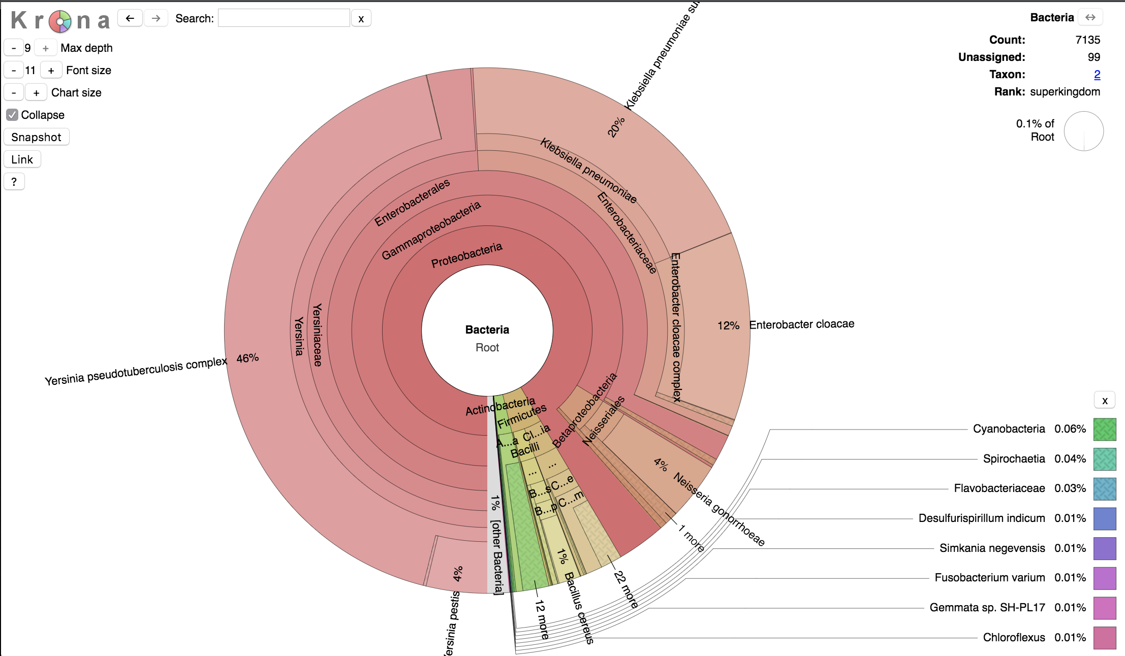
Finally, we can visualize the results of the Kraken2 analysis with Krona, which disaplys hierarchical data (like taxonomic assignation) in multi-layerd pie charts. The interactive charts created by Krona are in the html format and can be viewed with any web browser. We will convert the kraken output in html format using the program ktImportTaxonomy, which parses the information relative to the query ID and the taxonomy ID.

ktImportTaxonomy -q 2 -t 3 filename.krk -o filename.krk.html

Some of the options available in ktImportTaxonomy:

Option	Function
-q <integer>	Column of input files to use as query ID.
-t <integer>	Column of input files to use as taxonomy ID.
-o <string>	Output file name.

Note

If you want to analyze multiple kraken files from various samples you view the results in one single html file running ktImportTaxonomy as follows:

ktImportTaxonomy -q 2 -t 3 filename_1.krk filename_2.krk ... filename_n.krk -o all_samples.krk.html

An alternative tool for visualising the results of Kraken2 is Pavian, which analyses the file.krk output. You can run Pavian in R after installation or directly in the web server, as explained in the manual.

Once visualized our results, you can move to the estimation of taxa abundances with Bracken.

3.1.3. Kraken2 Custom Database

We have already created a custom database to use in this hands-on session so we can go straight to the next step (Taxonomic profiling with Bracken). However, we report here all the commands to build a Kraken2 database (steps 1-3).

The first step is to create a new folder that will contain your custom database (choose an appropriate name for the folder-database, here we will call it CustomDB). Then we have to install a taxonomy. Usually, you will use the NCBI taxonomy. The following command will download in the folder /taxonomy the accession number to taxon maps, as well as the taxonomic name and tree information from NCBI:
```
kraken2-build --download-taxonomy --db CustomDB
```
Install one or more reference libraries. Several sets of standard genomes (or proteins) are available, which are constantly updated (see also the Kraken website).
- archaea: RefSeq complete archaeal genomes/proteins
- bacteria: RefSeq complete bacterial genomes/proteins
- plasmid: RefSeq plasmid nucleotide/protein sequences
- viral: RefSeq complete viral genomes/proteins
- human: GRCh38 human genome/proteins
- fungi: RefSeq complete fungal genomes/proteins
- plant: RefSeq complete plant genomes/proteins
- protozoa: RefSeq complete protozoan genomes/proteins
- nr: NCBI non-redundant protein database
- nt: NCBI non-redundant nucleotide database
- env_nr: NCBI non-redundant protein database with sequences from large environmental sequencing projects
- env_nt: NCBI non-redundant nucleotide database with sequences from large environmental sequencing projects
- UniVec: NCBI-supplied database of vector, adapter, linker, and primer sequences that may be contaminating sequencing projects and/or assemblies
- UniVec_Core: A subset of UniVec chosen to minimize false positive hits to the vector database
You can select as many libraries as you want and run the following command, which will download the reference sequences in the folder /library, as follows:
```
kraken2-build --download-library bacteria --db CustomDB
kraken2-build --download-library viral --db CustomDB
kraken2-build --download-library plasmid --db CustomDB
kraken2-build --download-library fungi --db CustomDB
```
In a custom database, you can add as many fasta sequences as you like. For exmaple, you can download the organelle genomes in fasta files from the RefSeq website with the commands wget:
```
wget ftp://ftp.ncbi.nlm.nih.gov/refseq/release/mitochondrion/mitochondrion.1.1.genomic.fna.gz
wget ftp://ftp.ncbi.nlm.nih.gov/refseq/release/mitochondrion/mitochondrion.2.1.genomic.fna.gz
```
The downloaded files are in compressed in the gz format. To unzip them run the gunzip command:
```
gunzip mitochondrion.1.1.genomic.fna.gz
gunzip mitochondrion.2.1.genomic.fna.gz
```
Then you can add the fasta files to your library, as follows:
```
kraken2-build --add-to-library mitochondrion.1.1.genomic.fna --db CustomDB
kraken2-build --add-to-library mitochondrion.2.1.genomic.fna --db CustomDB
```
Once your library is finalized, you need to build the database (here we set a maximum database size of 8 GB (you must indicate it in bytes!) with the --max-db-size option).
```
kraken2-build --build --max-db-size 8000000000 --db CustomDB
```
Warning

Kraken2 uses two programs to perform low-complexity sequence masking, both available from NCBI: dustmasker, for nucleotide sequences, and segmasker, for amino acid sequences. These programs are available as part of the NCBI BLAST+ suite. If these programs are not installed on the local system and in the user’s PATH when trying to use kraken2-build, the database build will fail. Users who do not wish to install these programs can use the --no-masking option to kraken2-build in conjunction with any of the --download-library, --add-to-library, or --standard options; use of the --no-masking option will skip masking of low-complexity sequences during the build of the Kraken2 database.

The kraken2-inspect script allows users to gain information about the content of a Kraken2 database. You can pipe the command to head, or less.
```
kraken2-inspect --db path/to/dbfolder | head -5
```

Finally, we can run the classification of the reads against the custom database with the kraken2 command:

kraken2 --db CustomDB filename.fastq.gz --gzip-compressed --output filename.kraken --report filename.report

To visualize the results of the classification in multi-layerd pie charts, use Krona, as described in the section 3.1.2: Visualization of data with Krona and Pavian

3.1.4. KrakenUniq

Recently, a novel metagenomics classifier, KrakenUniq, has been developed to reduce false-positive identifications in metagenomic classification. KrakenUniq combines the fast k-mer-based classification of Kraken with an efficient algorithm for assessing the coverage of unique k-mers found in each species in a dataset. Basically, KrakenUniq reports an estimate of the number of distinct k-mers associated with each taxon in the input sequencing data. This allows users to better determine if Kraken’s classifications are due to reads distributed throughout a reference genome, or due to only a small segment of a reference genome (and therefore likely false positive). On various test datasets, KrakenUniq gives better recall and precision than other methods and effectively classifies and distinguishes pathogens with low abundance from false positives in infectious disease samples. The KrakenUniq function is implemented in Kraken2 by using the --report-minimizer-data along with --report:

kraken2 --db $DBNAME --report k2_report.txt --report-minimizer-data --output k2_output.txt sequence_data.fq

This will put the standard Kraken 2 output in filename_output.txt and the report information in filename_report.txt. Within the report file, two additional columns are present. The fourth and fifth column, respectively represent the number of minimizers found to be associated with a taxon in the read sequences (e.g. 1688), and the estimate of the number of distinct minimizers associated with a taxon in the read sequence data (e.g. 18). So for example if 182 reads were classified as belonging to H1N1 influenza, only 18 distinct minimizers led to those 182 classifications.

3.2. Bracken

Kraken2 classifies reads to the best matching location in the taxonomic tree (taxonomic binning), but they do not estimate abundances of species (taxonomic profiling). To do that we will use Bracken (Bayesian Reestimation of Abundance with KrakEN), which estimates the number of reads originating from each species present in a sample. Bracken computes probabilities that describe how much sequence from each genome in the Kraken database is identical to other genomes in the database, and combine this information with the assignments for a particular sample to estimate abundance at the species level, the genus level, or above. Bracken is compatible with both Kraken and Kraken2 (just note that the default kmer length is different, 31 in Kraken, 35 in Kraken2).

3.2.1. Taxonomic profiling with Bracken

Prior to abundance estimation with Bracken, each reference genome contained in the Kraken database is divided into “read-length kmers”, and each of these read-length kmers are classified. To do that, we need the library and taxonomy folders of the kraken database that we used for classification. This will generate a kmer distribution file, for examples for read-length kmers of 100 nucleotides: database100mers.kmer_distrib. The kmer distribution file will be used to reassign the unclassified reads. To do that, the length of the kmers in the distribution file should approximate the average length of the reads in your fastq files. You can generate “read-length kmers” of different sizes with the command bracken-build (see below). For the database that we used, customkraken2_2Gb_Feb2023_db, three kmer distribution files have been built at 70, 95, 130 kmers. To estimate the average length of the reads contained in your fastq files (just do that on one or two files) you can this (long) command:

zcat filename.fastq.gz | awk 'NR%4==2{sum+=length($0)}END{print sum/(NR/4)}'

To run Bracken on one sample we use the following command, with a threshold set at 50, and the read length set at 70 (so as to use the database70mers.kmer_distrib file inside the customkraken2_2Gb_Feb2023_db db folder). We will generate taxonomic abundances at the species level (the default option), otherwise use the option -l.

bracken -d path/to/Kraken2_v1_8GB -i sample.kraken.report -o sample.bracken -r 70 -t 50

Option	Function
-i <string>	Kraken report input file.
-o <string>	Output file name.
-t <string>	Threshold: it specifies the minimum number of reads required for a classification at the specified rank. Any classifications with less than the specified threshold will not receive additional reads from higher taxonomy levels when distributing reads for abundance estimation.
-l <string>	Classification level [Default = ‘S’, Options = ‘D’,’P’,’C’,’O’,’F’,’G’,’S’]: it specifies the taxonomic rank to analyze. Each classification at this specified rank will receive an estimated number of reads belonging to that rank after abundance estimation.
-r <string>	Read-length kmer used for the generations of Bracken distribution files

To speed-up the process, we can also use shell variables to set up the options and the paths to the kraken2 database and other folders, and a for loop. Also note that you can set as path variables either relative paths (based on your actual position and path) or absolute paths:

KRAKEN_DB=/path/to/kraken/db-folder
READ_LEN=70
THRESHOLD=50

for i in $(find -name "*krk.report" -type f)
do
  FILENAME=$(basename "$i")
  SAMPLE=${FILENAME%.krk.report}
  bracken -d $KRAKEN_DB -i $i -o ${SAMPLE}.${READ_LEN}mer.bracken -r $READ_LEN -t $THRESHOLD
done

The Bracken output file is tab-delimited. There are seven fields, from left to right:

Name

Taxonomy ID

Level ID (S=Species, G=Genus, O=Order, F=Family, P=Phylum, K=Kingdom)

Kraken Assigned Reads

Added Reads with Abundance Reestimation

Total Reads after Abundance Reestimation

Fraction of Total Reads

3.2.2. Build Bracken files

We used here pre-generated kmer_distrib files at length 70, 95 and 130. To generate different length files (and other Bracken database files) the command bracken-build is used. To do that, we need the library and taxonomy folders of the Kraken2 database that we used for classification. You can select the “read-length kmers” that is most suitable for your samples (namely the average insert size of your library, e.g. 60 bp for ancient libraries). You can also generate several kmer_distrib files and make different runs. You can find all the steps for generating the Bracken database files in the Bracken manual.

Warning

The library and taxonomy folders are big, but do not delete them if you plan to generate Braken databases in the future at different “read-length kmers”.

3.3. Mataphlan 3

MetaPhlAn is a computational tool that relies on ~1.1M unique clade-specific marker genes identified from ~100,000 reference genomes (~99,500 bacterial and archaeal and ~500 eukaryotic) to conduct taxonomic profiling of microbial communities (Bacteria, Archaea and Eukaryotes) from metagenomic shotgun sequencing data. MetaPhlAn allows:

unambiguous taxonomic assignments;

an accurate estimation of organismal relative abundance;

species-level resolution for bacteria, archaea, eukaryotes, and viruses;

strain identification and tracking

orders of magnitude speedups compared to existing methods.

metagenomic strain-level population genomics

We are not going to cover to in detail MetaPhlAn, but this is a great tool given its specificity, in particular to confirm the detection of peculiar microbial species (e.g. pathogens).

Warning

Please note that MetaPhlAn may have been installed in a separate environment that we called metaphlan. In that case, if you are already working in a conda environment, get out of it with conda deactivate, and activate the metaphlan environment conda activate metaphlan.

The basic usage of MetaPhlAn for taxonomic profiling is:

metaphlan filename.fastq(.gz) --input_type fastq -o outfile.txt

Note

MetaPhlAn relies on BowTie2 to map reads against marker genes. To save the intermediate BowTie2 output use --bowtie2out, and for multiple CPUs (if available) use --nproc:

metaphlan filename.fastq(.gz) --bowtie2out filename.bowtie2.bz2 --nproc 5 --input_type fastq -o output.txt

The intermediate BowTie2 output files can be used to run MetaPhlAn quickly by specifying the input (--input_type bowtie2out):

metaphlan filename.bowtie2.bz2 --nproc 5 --input_type bowtie2out -o output.txt

For more information and advanced usage of MetaPhlAn see the manual and the wiki page. And, recently, MetaPhlAn 3 has been released!

3.4. Other tools

We remind you that there are several metagenomic classifiers, all with their pros and cons, as discussed in the lecture. Other tools that we want to suggest are MALT (and the HOPS pipeline to analyse the data), and Centrifuge, which both implement alignment-based methods to classify the reads.